
One of the challenges synchronization engineers and technicians often face in the field, is the lack of proper Frequency and Time (Phase) references required for 1PPS Accuracy and Stability verification at remote sites. This leaves them with one practical choice: The use of portable GNSS-disciplined reference clocks.
Time (Phase) Holdover has also been proposed as an alternative reference to help with indoors testing (no GNSS signal). It is important to understand how it works, its limitations and how to use it properly, to have a clear and practical idea of what to expect and what not.
Wherever there is access to accurate, stable and traceable frequency and timing references, use them!
GNSS, GPS in particular, is the best (if not the only practical) option available to get accurate time and frequency almost anywhere in the world. But it is not perfect. Knowing the GNSS limitations helps in defining correct test procedures and setting realistic expectation for field testing.
This article includes simple explanations on how disciplining and holdover work, so it benefits a greater audience, including field engineers and technicians who are new to synchronization. Nevertheless, experienced individuals should not be discouraged from reading through, since some of the information bits may “strike a note” and/or encourage participation in discussions and contribute to improving the information currently available, as well as combat a great deal of misinformation and bias floating around.
1. Basic Disciplining Introduction
Basically, a GNSS-disciplined Clock consists of a high-quality oscillator that is continuously being corrected using the coordinated universal timing signal (UTC), or standard second, in the form of 1PPS pulses recovered from the GNSS/GPS signals. In theory, the rising edge of the One-Pulse-Per-Second (1PPS) represents the beginning of a standard second all over the world (in practice it is very close).
Frequency and Phase are tightly related, but don't assume that having accurate frequency guarantees accurate phase. In that sense, they are quite different. A disciplining control system will actually make its frequency source inaccurate, on purpose, in order to achieve and maintain accurate phase (Time). There is also noise, jitter and wander in an otherwise perfect frequency source which cause random (phase) walk.
1.1 Relationship Between Frequency and Phase
Imagine that a frequency of 1 GHz (1 ns cycle) is used for this simplified example, to make mental and visual calculations easier. The illustration depicts the relationship between Frequency Offset and Phase Drift, which are used in the 1PPS disciplining process to control the rising edge position of the output pulse, relative to the standard second. The darker cycles indicate the end of the billionth cycle.
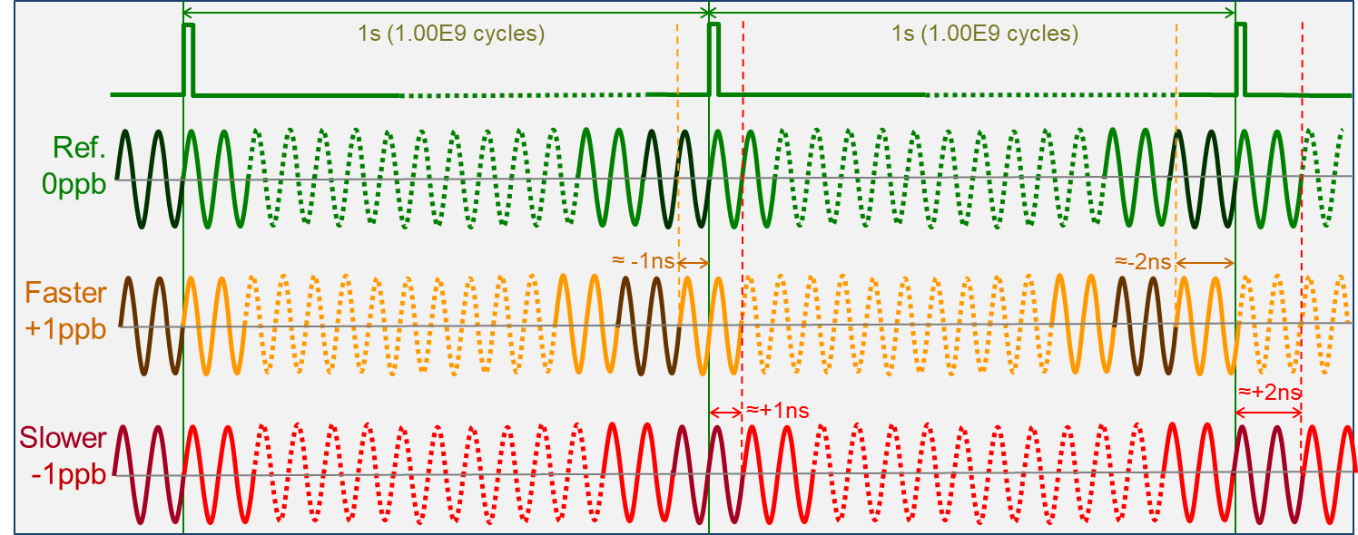
If a 1,000,000,000 counter is used to count one second and the frequency is 1,000,000,001 Hz (+1 ppb or +1E-9), the counter would roll over ≈+1 ns earlier, adding about 1 ns of Time Error (TE) for every second that goes by (cumulative). It is similar for 999,999,999 Hz (-1 ppb) as the counter would roll over ≈-1 ns later, then -2 ns, -3 ns, etc. That is, positive frequency offset creates positive phase drift (TE) and negative frequency offset creates negative phase drift, at a rate of X ppb ≈ X ns/s.
We can see that, when looking at it at the nanosecond, even the smallest frequency error can result in significant Time Error (TE) drift. For example, a clock with ±1 ppb (1E-9), would drift ±1 ns every second (that is ±100 ns in one minute and 40 seconds!). A typical portable atomic clock, such as those used for field testing, with a free-running frequency accuracy of 10 parts-per-trillion (1E-11), or 10 ps/s, would drift to a 100 ns Time Error in just 2 hours, 46 minutes and 40 seconds (10,000s).
1.2 Simplified Frequency Disciplining Explanation
To correct any frequency deviation (offset) in a local oscillator, the system basically counts the number of cycles that occur between the rising edges of two consecutive 1PPS reference pulses (i.e., "exactly" one second). If it is a 10 MHz oscillator and 10,000,010 cycles are counted, then the oscillator is running 1 ppm (1E-6) too fast. Then the control system would change (steer) the oscillator's frequency to slow it down. It counts again and gets 10,000,001 cycles, indicating that the oscillator is now running with 0.1 ppm offset and uses it to make another correction to perhaps get 9,999,999.9 (-0.01 ppm). Then finer and finer corrections are made, until the count is as close to 10,000,000 cycles as the system can measure, hence achieving a very high frequency accuracy (e.g., in the order of parts-per-trillion, or 1E-12). It continues making those very small corrections to compensate for any changes due to ambient temperature variation and oscillator's ageing. Basically, the oscillator is being "soft" calibrated, and it should now be highly accurate and stable. That sounds easy.
One of the caveats here is that the 1PPS timing reference recovered from GNSS is not ideal. It is real and it has to deal with our imperfect world (e.g., ionospheric and atmospheric changes). That otherwise "perfect" second varies (wanders) over time. It means that some of the frequency measurements made by the disciplining control system would be off and slightly wrong correction calculations would be made. Disciplining systems mitigate this problem by applying some statistical algorithms before issuing the steer correction to the oscillator. Having a high-quality oscillator would also help as they are difficult to steer, creating a dampening effect that helps filter the noise (errors). The end result is a frequency source that benefits from the best of both worlds. The short-term stability of a good oscillator plus the long-term accuracy of GNSS equals a highly accurate and stable frequency source.
For extra details, refer to the video below:
1.3 Simplified Phase (Time, Timing) Disciplining Explanation
The process is very similar to older frequency-only GPS Clocks described earlier, but in this case the priority is to keep the 1PPS phase aligned to the beginning of the standard second (not its frequency). That is, the control system intentionally changes the frequency of the oscillator to keep the 1PPS phase aligned to the standard second (UTC). As one could imagine, some frequency purists may not like this approach, at first. Imagine starting with a perfectly calibrated 10MHz oscillator and the first thing the disciplining control system does is to deliberately change its frequency to move the rising edge of the 1PPS pulse closer to its ideal position.
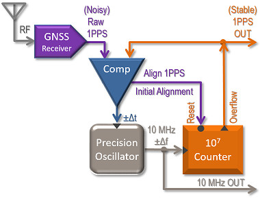
If the output of the disciplined 10 MHz oscillator described earlier is fed to a 10,000,000 counter, it will produce an overflow pulse every time it rolls over from 9,999,999 to zero. That is, one pulse per second (1PPS). Initially the position of the resulting 1PPS output is arbitrary, so the first task for the phase disciplining control system is to perform a rough alignment by using the GNSS/GPS 1PPS pulse to reset the counter. This leaves the output 1PPS within 100 ns (or one 10 MHz cycle) from the standard UTC second. To fine tune the 1PPS phase alignment to UTC, the control system has to slowly change the oscillator's frequency. For example, if the local 1PPS is 50ns late, the frequency of the oscillator is slightly increased to count faster and start reducing the phase error (or Time Error). On the other hand, if the local 1PPS happens before UTC (e.g., -25 ns), the oscillator is slowed down to delay the counter. It could be said that the amount of new frequency offset corrections are proportional to the remaining Time Error (plus some amount of vendor-specific statistical magic). It means that the local phase should slowly converge towards UTC and the amount of frequency offset (inaccuracy) in the output reduces. Once this convergence happens, the GNSS Clock should be outputting fairly accurate and stable 1PPS timing and 10 MHz frequency references.
In the absence of any other references or instruments, field users should monitor the ±Δt value (internal phase error) to identify when the disciplining has converged (horizontal trend at around 0ns). At that point, the test set should have reached the best accuracy it could possibly get under the existing conditions.
Why don't just use the 1PPS directly from the GNSS Receiver?
- First, it is quite noisy (jittery) and needs to be stabilized.
- Second, it could go away at any time, so a good local oscillator is required to help bridge any outages (holdover).
For further details, refer to the video below:
2. Using GNSS Disciplined Clocks for Field Testing
High quality GNSS-Disciplined Clocks (PRTC) are excellent timing sources and frequency references for:
- Frequency accuracy (Offset) and stability measurements (Wander)
- 1PPS phase accuracy (current Time Error), short-term and long-term Timing stability measurements (Wander), PTP 2WayTE, etc.
- One-Way Delay (Latency) and Asymmetry measurements.
Keep in mind that not all GNSS Receivers are necessarily good GNSS Clocks. Even within the GNSS clock category, there are different quality classes, in part due to the type of local oscillators they use: Cs, Rb, DOCXO, OCXO or even TCXO. The oscillator's quality plays a key role in the GNSS Clock performance required for test and measurements, especially when considering Holdover performance.
When performing frequency-related tests, such as wander (TIE, MTIE, TDEV), cable lengths may have not been an issue. However, with Time Error measurements the situation is completely different. Every meter of cable introduces about 5 ns of delay (error) which can add up very quickly.
- The antenna cable delay must be properly documented and programmed into the GNSS receiver for 1PPS delay compensation.
- Test cables (from DUT and 1PPS reference) must be of the same length to cancel out their respective delays, otherwise their specific delay compensation values (in ns) must be entered in the test equipment.
2.1 Selecting the Right Disciplining Parameters
Sometimes test equipment users may not have any options, as the vendor selects them and don't provide (or disclose) any of the settings for it. However, there is a value in being able to modify GNSS Survey and Atomic Clock Disciplining, to tailor them to different applications, requirements and even time constraints. For example, if one needs to perform quick (short-term) long distance One-Way Delay (OWD) measurements with 1 μs or 1 ms resolution or similar accuracy, then it may make sense to relax those windows to lock the GNSS and Atomic Clock faster. However, it is important to experiment and know the behaviors before making an such informed decision.
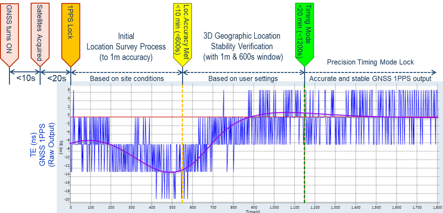
- Total System Lock Time = GNSS Survey Time + Atomic Clock Disciplining Time
For precision timing GNSS receivers, the Survey time could vary depending on several reasons (e.g., RF quality, satellite visibility, constellations, bands, etc.). VeEX users have control of the 3D Location Error allowance and the evaluation Window. One could increase the location error to 5m and reduce the evaluation window to a couple of minutes, to shorten the total survey time, but that would also compromise the position accuracy and hence the accurate time calculations. The GNSS lock time may also be longer if it is the first time that the receiver is being used at a new location, since it needs to gather more information from the available satellites.
- For VeEX Instruments, using Single or dual-band, dual or quad-constellation receivers, we recommend sticking with 1m threshold and 600s (10 min) evaluation window, when good satellite signal is available.
In the case of Atomic Clock Disciplining, larger Time Constants (TC) make the clock more difficult to steer. So, in theory, more stable or impervious GNSS variations. However, with modern very stable high-precision GNSS receivers (e.g., quad constellation, dual band), if the TC is too large, the Atomic Clock's natural frequency may prevail over the GNSS corrections. That is, the GNSS may not have the "power" to correct the hard-to-steer clock and the 1PPS output may end up drifting quite a bit. Although the frequency error could be <±5E-11, it could accumulate significant amounts of TE over long-term measurements.
- In the case of VeEX instruments, with built-in Atomic Clock and high-precision Quad-constellation Dual-band Receivers, for long-term measurements the recommended TC = 1800s, with a time error threshold of 50 ns.
2.2 Total Test Time Expectations
As implied earlier, the total expected time required to run a precision timing measurement includes the necessary preparation time. GNSS survey and Atomic Disciplining are variable times.

Testing time varies depending on whether you are just checking the current Time Error or OWD (short), or you are looking at the long-term stability of the 1PPS clock source (e.g., 72 hours).
2.2.1 How much time does the GNSS Survey take?
The time it takes for the GNSS to lock into Precision Timing mode depends on different factors:
- If it is the first time it is used at a new geographical location, it needs to gather extra data from the satellites.
- Antenna location, number of constellations, bands and visible satellites.
- Satellite (RF) signal quality (C/No density).
- Once it can calculate location (coordinates) and time for the first time, it will improve its coordinates accuracy, until it meets the defined threshold (e.g., <1m).
- Then, it will wait for the assessment window to be met. For example, if the window is set as <1m for 600s, then it will take 10 minutes to validate the 3D accuracy and stability (as long as the deviation stays within <1m for the last 600s).
Here is one example for a survey window of 1m and 600s.
Recalling saved coordinates, from previous site surveys at that location, helps shortening the time required to achieve Precision Time lock.
For long term tests (e.g., 72-hour weekend) with roof antenna and full sky view, 1m and 600s is recommended. For a quick Time Error check or OWD measurements, once could use 3 to 5 meters and 60 to 300 seconds, to save time. For less-than-ideal satellite signal quality, users should just check what is the best location deviation that can be achieved on site and use a slightly larger threshold.
2.2.2 How much time does the Atomic Clock Disciplining take?
The clock disciplining time is also variable, as it depends on two main factors:
- The initial free-running frequency offset (error) of the oscillator. The bigger the deviation from its specified frequency, the longer it would take for the initial correction process.
- The disciplining validation window being used, which is in fact made of two parameters: Maximum allowed error threshold and validation time.
- Time Error Threshold (ns) - This is related to the target accuracy and short-term stability at the end of the process.
- Time Constant (s) - This is related to validating long-term stability. It defines the evaluation window (the amount of time the output time error must be less than the threshold, before declaring a lock) and sets the "stiffness" of the frequency steering mechanism. Longer time constants make the frequency change slower (smoother). If the discipline window is set to 20 ns for 1800s, the clock will only lock when the 1PPS output error stays below 20 ns for the past 30 minutes.
So, it will take certain amount of time for the clock to reach the correct its frequency and phase (e.g., <20 ns), plus at least one time constant (provided that the clock remains stable and/or converging to the ideal 0 ns target).
The following examples are measurements of the internal Atomic 1PPS against an external PRTC, to show the effects of different disciplining window settings.
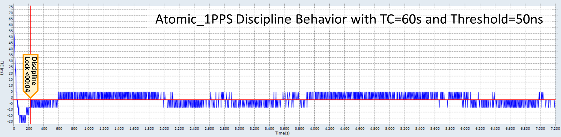

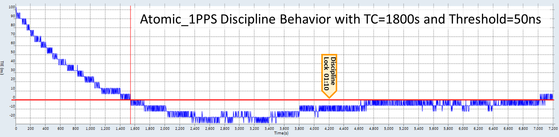
Even though TC=60s is much faster to converge to 0 ns, its loose steering is not recommended for long test or holdover applications. Larger TCs, like 1800s, offer a good compromise between convenience and assured stability for long-term tests.
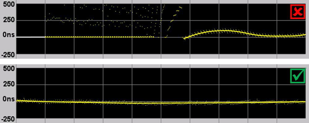
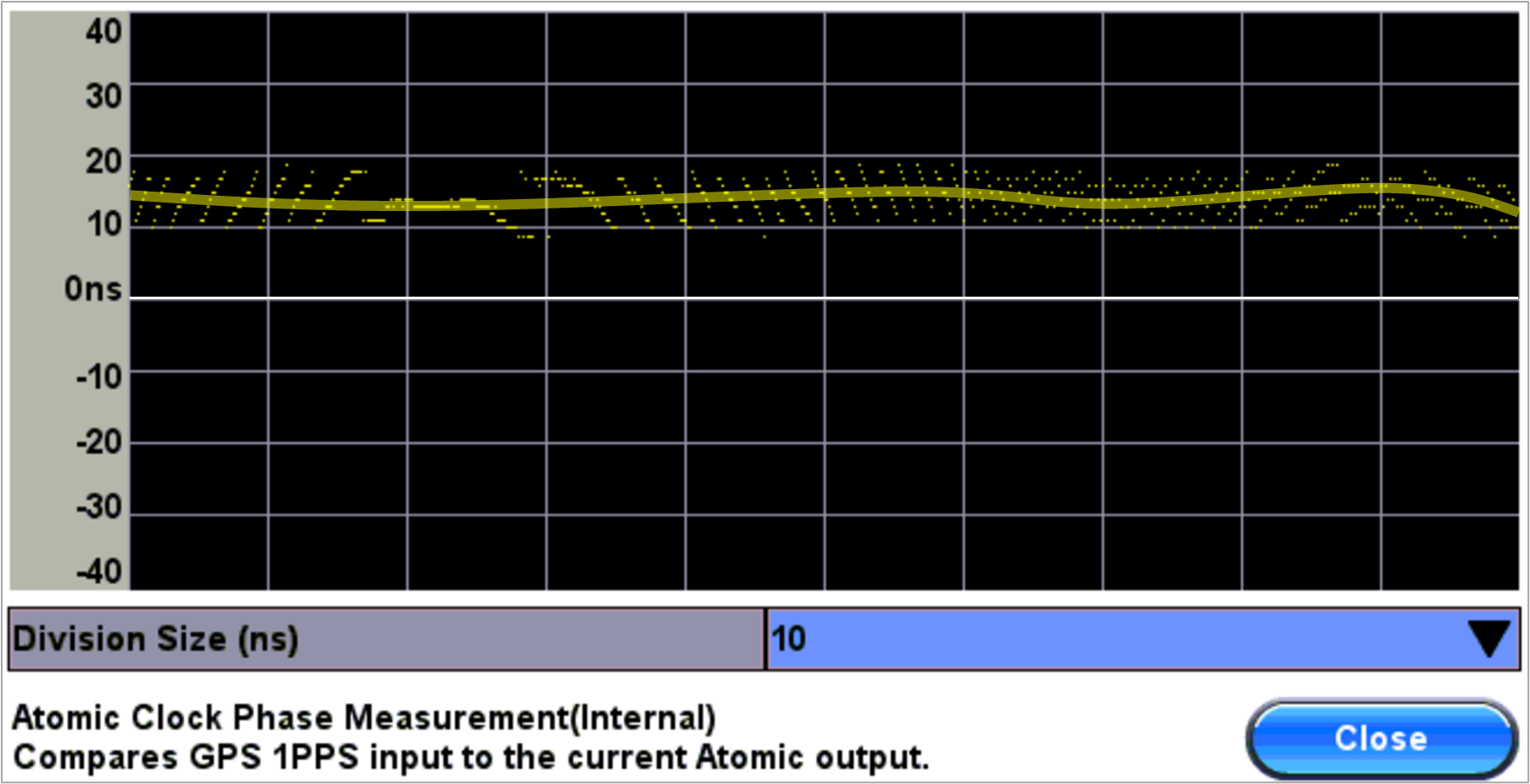
However, from the practical point of view, these graphs may not mean anything for field testing, because the only clock signal available on site may be the one you are trying to verify. Some solutions rely on a LOCK status message or icon on the screen, which sometimes may be misleading. For that reason, VeEX's products offer an insight view of the internal Phase Error ![]() of their Atomic Clocks, so users can make a more informed decision on whether to start the testing right away or wait a little bit longer. The graph below shows the internal Phase Error at the moment when the Atomic Clock (TC=1800s) displayed locked state. This 10-minute monitoring window clearly reflects the remining Time Error shown in the graph above. Otherwise, users would have operated "blindly".
of their Atomic Clocks, so users can make a more informed decision on whether to start the testing right away or wait a little bit longer. The graph below shows the internal Phase Error at the moment when the Atomic Clock (TC=1800s) displayed locked state. This 10-minute monitoring window clearly reflects the remining Time Error shown in the graph above. Otherwise, users would have operated "blindly".
3. Holdover Introduction
Although GNSS signals "rain" freely from the sky, they are quite faint, compete with other locally generated frequency sources (noise) and their own reflections (multi-path), have poor penetration and are easily obscured. They are not available (or reliable) indoors, in "urban canyons" or noisy RF environments. So being able to hold the last know frequency and timing during the GNSS outage becomes a key feature in stationary and outdoors applications. This is why GNSS receivers are paired with high-quality oscillators, to create clock sources with holdover characteristics that can bridge temporary outages. A feature the test and measurement community dreams of, and sometimes seem to elevate to "superpower" levels, since equipment rooms often lack GNSS connection or other traceable timing sources.
Unfortunately, those obscured places are the ones we need to run tests at (shielded cabinets, containers, base stations, central offices, equipment rooms, office buildings, basements, data centers, etc.). The proposed solution (or idea) is to extend the use of the atomic clock's holdover characteristics into becoming a temporary mean of transporting time synchronization from the outdoors to indoors. That is the dream.
One thing is using holdover to keep 5G radio units' (antennas) phase and frequency somewhat in sync, during a GNSS or PTP outage (e.g., Time Error under ±1,100ns for 24 hours, with a 1.27E-11 clock), but using it as a measurement reference is a completely different challenge. Even applying the simple old rule that instruments must be 10x more accurate than the device under test, would leave us with a ±100ns target. However, in the precision timing world, that would be considered too much uncertainty.
Before jumping into the holdover-for-testing explanation, keep in mind that the phase disciplining process constantly changes the oscillator's frequency to keep its 1PPS aligned to the standard UTC second. Even though those fine adjustments are in the order of parts-per-trillion, they affect the final holdover performance.
Most of the holdover data available is from controlled lab environments and controlled conditions. Many are based on using an accurate and very stable 1PPS from a PRTC, to discipline the atomic clock, instead of a noisier 1PPS from a GNSS receiver. Taking that knowledge to the field is a huge leap of faith.
Also, the Time Error graph (drift) behavior is unpredictable. One can run the same holdover Time Error vs. time multiple times and sometimes the error will go up, others down (negative), all with different slopes (frequency offsets).
3.1 Using Disciplining and Holdover in Field Test Applications
The following graph depicts the full Time Error (TE) cycle of a test set's internal 1PPS reference, starting from free running, disciplining, to holdover. The test was run in conditions similar to what field technicians would encounter at remote sites. The main difference is that we had access to a 1PPS reference (PRTC) and equipment to monitor and document the internal 1PPS behavior for this article, but field technicians won’t have the same luxury. That is the reason why it is important to carry reliable test instruments which provide as much information about their internal status and readiness as possible.
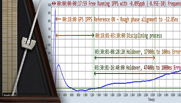
A test set, equipped with GNSS/GPS receiver and Chip-Scale Atomic Clock (CSAC) oscillator, was selected for the experiment. It was turned on and its internal GNSS-disciplined 1PPS reference was constantly recorded, but the TE information was not used for any decision making during the test. Let's interpret this graph one section at a time.
3.2 Free Running Stage
The initial part of the trace shows the internal 1PPS phase compared to the reference, while the GNSS disciplining function was still disabled (free running).
The first 1085 seconds of the TE trace indicate that the oscillator is very stable (straight line) but it has a free-run accuracy (frequency offset) of -0.895 ppb, which causes the phase to drift at a rate of 0.895 ns/s. The straight TE lines, which identify highly stable oscillators, make it easier to calculate their frequency offset by using simple math. Test sets can also perform the offset calculation, with the advantage that they can do it for more complex scenarios.
3.3 Disciplining Process
18 minutes later (1085s), with the GNSS/GPS already locked to satellites, the Atomic Clock Disciplining is enabled, and the disciplining process gets started. The first thing that happens is the internal 1PPS being forced to align with the 10 MHz cycle closest to the UTC second. In this case, the TE reads -12.5ns.
The first dot shows a trend indicating that the internal oscillator still wants to run at 9,999,999.99016Hz (10 MHz -0.895 ppb), after the initial rough phase correction. The disciplining control system starts to steer the oscillator into running faster and at the 2000s mark it reaches exactly 10,000,000 Hz (0.0 ppb). If the goal was to achieve frequency accuracy only, the process could have been stopped at this point and let it stay in that perfectly horizontal trend indicated by the dotted line. But the priority is Phase (Time) and 300ns error was accumulated in the process of getting to this point, which still need to be corrected. So, the process continues by making the oscillator run a little bit faster than its nominal value, in order to make the pulse’s phase drift to the “left” (as shown in the initial diagram).
The third dot (3000s) shows the oscillator running a bit faster at 10,000,000.001285 Hz (+0.1285 ppb) to reduce the phase error. As the 1PPS phase error approaches 0.0ns, the oscillator is slowed down to make it converge. Depending on the conditions, the whole process could take long time, which could be an issue for field testing, if not done correctly.
The fourth dot (at 12600s or 03:30:00) shows that the oscillator was running at 9,999,999.9999285 Hz (-0.00715 ppb) before the GNSS/GPS 1PPS reference was disconnected. That is two orders of magnitude better than its free-running frequency. At first, this may look impressive, but even in a controlled lab environment a 0.00715 ns/s phase drift rate would cause the accumulation of 100ns error in about 13,986s (03:53:06).
Also note that, after checking the internal phase graph to confirm that the disciplining process has stabilized, the point of disconnection is basically selected at random. No one can really guarantee what the exact frequency offset would be at every single occasion. It could be slightly larger or smaller, positive or negative, so there is a degree of uncertainty in the final holdover behavior. Keep in mind that field technicians don't have access to the measurements or calculations shown here, when making the decision to force the test set (or external reference) into holdover. So, having information about the internal disciplining process and status becomes very important.
3.4 Forcing the Test Set into Holdover
At the 12,600s (03:30:00) mark the GNSS/GPS was turned OFF (disabled), to force the test set's internal Atomic 1PPS reference into holdover mode, so one can enter the premises to perform Absolute Time Error, Wander or One-Way Latency measurements.
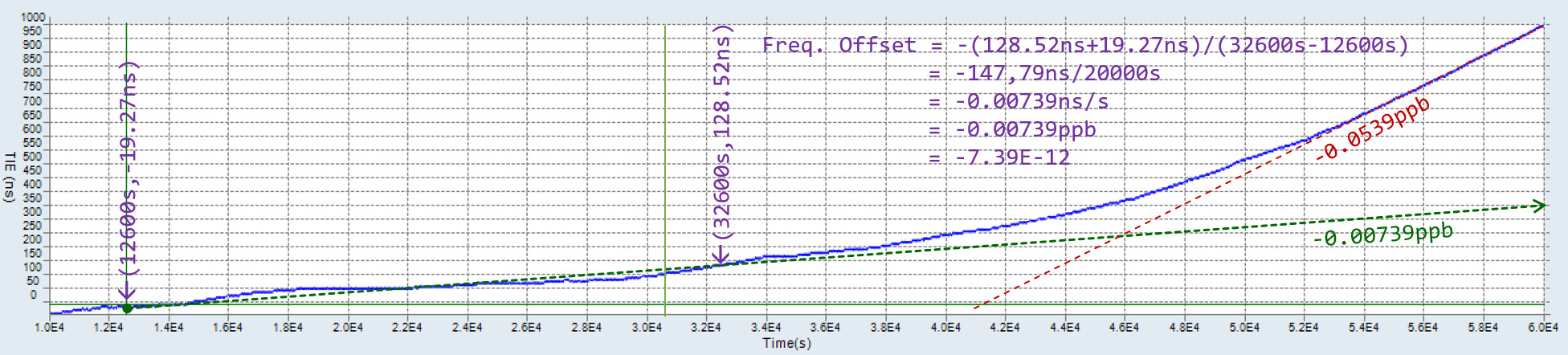
At an initial 0.00739 ns/s phase drift rate (7.39E-12), this initial trend is very close to what was calculated before the holdover was started. This confirms that the oscillator will keep the last frequency correction to try holding the last known time alignment. The first 100 ns error are accumulated after 17,900s (04:58:20) of holdover and the 1000 ns threshold is reached after 47,400s (13:19:00), but at this point the oscillator has already started to drift from its disciplined frequency, into its natural frequency.
3.4.1 Holdover Repeatability (or Lack Of)
It is important to know how the selected portable or built-in GNSS-disciplined Clock Source works, under those conditions specific to a network and its environment. As mentioned before, the total holdover time to certain amount of allowed uncertainty (or error) is mainly determined by (a) the frequency offset or correction applied to the oscillator at the moment the GNSS/GPS 1PPS is disabled or disconnected, (b) the stability of the oscillator, (c) internal and external temperature variations (d) phase noise and (e) Ageing. among other factors.
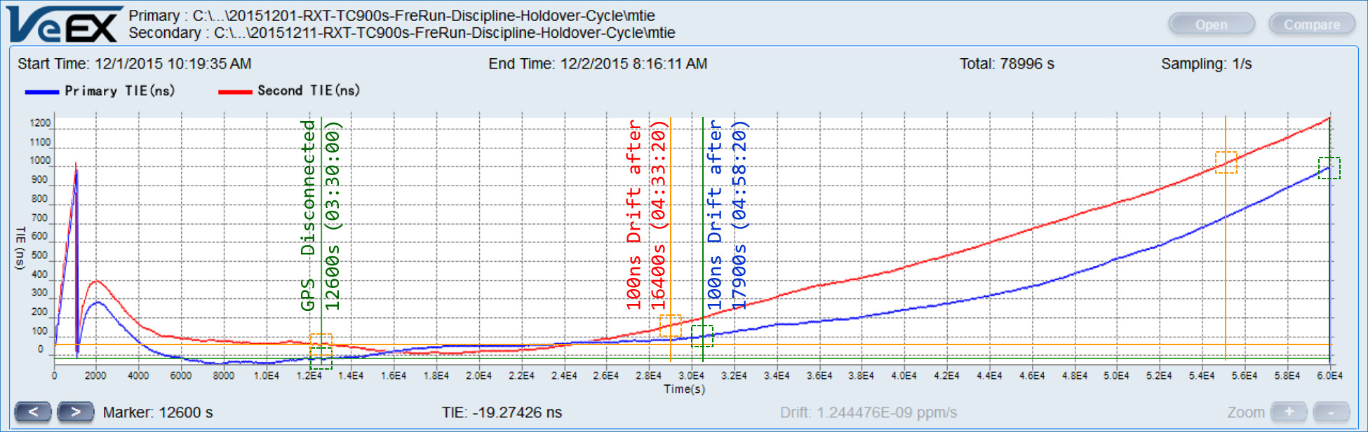
A week later, the same test set was used to run the same experiment again, using approximately the same times, to start the disciplining process and force the holdover. The graph shows the differences between the first (blue) and second (red) tests. Temperature and sky condition were slightly different since the second test was performed on a rainy day. That is good example of what real-life field conditions mean.
As expected, the two traces are slightly different. There is a baseline offset of about 70ns between the original and the new TE traces, which could be due to the internal GNSS Clock plus the external GNSS-disciplined reference (PRTC) uncertainties. Also, in the new test results (red) the first 100ns accumulate faster (25 minutes earlier) and it reaches the 1,000 ns mark earlier, after 42,000s of holdover.
If 100 ns uncertainty is considered acceptable, it could be said that this reference could be used for up to four hours in both cases, but field users need to be aware that disciplined oscillators don’t behave exactly the same every time. Also, there is not a good way to know how the clock holdover is behaving in real time, so this should be considered a major uncertainty. The behavior is not necessarily linear either.
3.4.2 The (Unpredictable) Effects of Temperature Variations

Most precision oscillators or clock performance parameters' specifications are given for (tested in) controlled constant-temperature (lab) environments, since precision oscillators are affected by temperature variations. Even oven-controlled oscillators get affected a bit by ambient temperature changes, but at the nanosecond scale, they can be significant. It is also important to remember the Time Error measurements not only measure the error from device under test (DUT), since it also includes any TE variations from the reference clock being used. Temperature changes could also come from the devices' internal heat dissipation.
The following example shows a holdover test performed with test equipment and PRTC reference in an office building, with a regular heat ventilation and air conditioning (HVAC) system. Two hours (7,200s) of disciplined behavior are recorded at the beginning to have a baseline of the system, then the GNSS is turned off and monitored for 22 hours.

It clearly shows the non-linearity introduced by significant temperature changes when the HVAC turned OFF overnight and turned back ON in the morning. However, when the HVAC turns OFF, it seems like the Atomic Clock's holdover had already started to diverge towards its calibrated free-running frequency (-1.86 ppt). So, if the temperature had not changed, it would have followed the purple dotted line. The same (orange) slopes show up when temperature stabilizes overnight and then when temperature stabilizes after the HVAC turns back ON. In this particular example, the first temperature change gave it a correction boost (non-linear however), extending the time to reach the ±100 ns Max|TE| threshold. These conditions should be taken into account when creating or executing Time Error test procedures that call for internal reference clock in holdover mode. That also includes the potential temperature shock that can occur when disciplining outside (with good satellite reception) and moving inside to test using holdover mode.
If that clock's holdover was to be used for One-Way Delay measurement with microseconds resolution or accuracy, the results would have been fairly good for about 20 hours. However, if it was to be used for PRTC or PTP TE verification, with nanosecond granularity, the holdover would have only been good for about two to three hours.
3.5 Using Forced Holdover for Testing
As a general rule, the use of phase holdover for testing should only be considered as an alternative for those occasions when GNSS/GPS coverage is not available. If good GNSS signals or any other traceable accurate 1PPS reference are available on site, use them.
In this particular case one could say that the test set could be able to perform fairly accurate Time Error and Wander measurements within four hours of entering into holdover mode, and One-Way-Delay for at least eight hours (assuming 1μs accuracy and resolution). But that may not always be the case. Results will vary depending on the disciplining settings, satellite signal quality and environmental conditions.
Don't forget that the GNSS receiver used to discipline the oscillator also has its own time error, which may vary depending on atmospheric and ionospheric conditions, as well as antenna placement and temperature variation. So, there is an uncertainty to start with (100 ns allowed for GNSS per ITU-T G.8272 clauses 6.1 and 6.2, although modern quad-constellation dual-band receivers can offer much better accuracy and stability).
Another issue to consider is the amount of time the GNSS Clock takes to discipline to achieve its most accurate and stable frequency and phase. Three hours may be considered too much of a wait for a field test or even impractical to some. There are ways to make it synchronize faster, but not without some tradeoffs. This is why it is important to fully understand the concept, so practical guidance, procedures and expectations are put in place to achieve the desired goals. Here are some examples:
- Reduce the GNSS Clock's location survey assessment window or increase the allowed location error, to make the receiver lock faster (but with less accuracy).
- Reduce the Atomic Clock's Time Constant or its error threshold allowance, to make the disciplining control system react faster and converge quicker. However, this may reduce the stability of the 10MHz and 1PPS output, affecting (reducing) the holdover time.
- Use the GNSS Receiver's status information (satellites and their Carrier-to-Noise Density, C/No) to make sure the temporary portable antenna installation is good and assure the best RF reception possible. Watch out for potential multipath reflections caused by tall buildings and reflective glass. Go to the roof-top, if necessary.
- Some stand-alone GNSS Clocks may turn on their green Lock light long before they achieve their best accuracy. Monitor the Altitude or Elevation to make sure it is no longer changing (no longer in site survey mode), and its value makes sense for where you are at. We have found that this could be a good indication that the GNSS survey has identified its most accurate position and can now calculate time accurately.
- When expecting to visit the same site multiple times, it is recommended to perform a very accurate site survey and save the final coordinates. Next time you visit the site, you can reload the coordinates and save a lot of time (no site survey required).
- Use the latest GNSS receiver technology available to assure getting the most accurate and stable time (e.g., Quad-constellation dual-band receivers can see much more satellite signals and can compensate for ionospheric variations).
- In some cases, you may be able to start the survey and/or disciplining process as you drive to the site. By itself this is not recommended, but in certain conditions it could help in getting a good part of the process going, potentially reducing the amount of stationary disciplining time left to achieve the required accuracy. Do not try this with stand-alone GNSS Clocks as they may be set for stationary operation.
- Monitor the internal oscillator's Phase Alignment graph to get an idea of when it has reached an agreement with the GNSS receiver and has become stable. A horizontal trend around 0ns would be a good indication that it may be safe to initiate the holdover. Keep in mind that this is internal indication is relative, since there may not be any other references to compare it to.
- Do not disable disciplining function to force the equipment into holdover. Instead disable or turn off the GNSS receiver side. However, if no other options are available, disconnect the antenna. Switching the disciplining function from ON to OFF may change some parameters in the oscillator and affect the corrections previously made by the disciplining process.
- Consider leaving some margin for all the uncertainties, when measuring Absolute Time Error. For example, 50ns for the GNSS receiver, 10ns for the disciplined clock and 100ns for the holdover drift. If the limit is ±1,100ns, perhaps the internal goal could be set to a ±800ns Pass/Fail threshold. (These numbers are presented for illustrative purposes only. This is not a specific recommendation.)
- Set reasonable test time limits. Not too short that TE or TIE traces could become misleading and not so long that too much holdover error accumulates.
- At about 5ns/m (1.5ns/ft), any significant cable-induced delays must be accounted for in the test setup, especially the antenna cable. If a local or portable reference (Cs or Rb) is used, make sure the cables carrying the reference signal and signal under test are of the same length, to cancel their respective delays, or better yet, enter their respective delays in the compensation fields.
- Learn about the oscillator technology used in the selected Frequency and Time reference. Identify and document its requirements: Warm up, temperature, overnight and long-term storage, handling (shock/vibration), calibration requirements and how to keep it in top performance. Then add "Equipment Handling Guidelines" to field test procedures.
- Visit and understand different typical sites, in which measurements will be performed, so test procedures align with the reality end users (field technicians) will be facing.
- Training the work force is very important. After all, phase could be a concept new to them. Understand experience levels and training needs for the field crews who will be performing these verification tests. Do they have frequency sync experience? Do they need phase/timing/time synchronization training?
4. Conclusion
When properly understood and used correctly, GNSS (GPS) Disciplined Oscillators and Holdover are indeed powerful tools which enable Phase and Frequency accuracy and stability measurements in places that would otherwise be impossible or cumbersome to test, due to the lack of local references. End users should become familiar with this technology and understand the way it works, in order to use it properly, achieve the best performance and obtain valid results. Training is one of the most important aspects for verifying Time Error in the field.
Instruments and references used in remote sites should provide detailed status information about their GNSS receiver, oscillator and disciplining process. After all, that may be the only information field crews may get to assess the instrument’s readiness or decide when to initiate a successful holdover, if required.
If any user decides to use holdover as a reference for testing, they should be kept short, to limit the reference time error accumulation. Holdover should not be used for long term testing, only for quick Time Error checks. Perhaps consider keeping the holdover for less than one hour to try limiting the accumulated error below ±100ns. If measuring One Way Delay (OWD) in the order milliseconds or microseconds, then users may be able to afford longer tests and longer uncertainty, due to the larger scale.
Implement practical test procedures that fit the local needs and requirements, with end users in mind. Set practical limits and realistic expectations.
This article was originally published in 2015 and it has been updated over time.