Can Constant Time Error (cTE) Dynamic Time Error (dTE) be Measured?

A Practical Approach to Understanding TE=cTE+dTE in Precision Timing Applications

Introduction

In early 2016 we started receiving many questions about the usefulness of cTE (constant Time Error) and dTE (dynamic TE), which come from the overly simplified expression:

TE = cTE + dTE.

Its application for development and validation of network elements and clocks was fully understood and justified. However, they suddenly seemed to have become must-have measurements or required test parameters around the world, to qualify actual 1PPS clock outputs outside of lab environments. Apparently, they were being promoted as very important requirements to qualify PTP networks, links, nodes, network elements and other timing reference equipment, in the field.

Given the opportunity, it is always good to (respectfully) ask end users if they fully understand the application or true value added of whatever measurement, parameter or buzzword is in season. As you may imagine, the answers or justifications are not often encouraging. Sometimes people have the tendency to repeat whatever they heard at the last seminars, webinar, trainings or even sales pitches. Sometimes, certain vendors may use scare tactics (a very technical form of marketing terrorism) to persuade customers to buy, replace or upgrade their equipment.

The purpose of this paper is to explore the “true” meaning of cTE and dTE, applied to physical 1PPS clocks, from a practical point of view (it can also be extended to packet-based measurements, like 2WayTE). It is important to understand what they really are, to figure out how much value they can add. In other words, put TE, cTE and dTE in perspective, by using actual data and avoiding any theoretical simulations or made-up drawings.

Where do cTE and dTE come from?

In general, any physical behavior may be represented as:

y(t) = C + K∙t + d(t) + n(t)

In which C is a constant component (e.g., physical phase delay), K∙t is a linear behavior (e.g., drifting effects due to constant frequency offset), D represents a non-linear behavior (e.g., effects of frequency drift) and N is random noise (e.g., oscillator stability, temperature, PDV, phase noise, etc.). In that sense, the absolute Time Error of a 1PPS signal could be expressed as:

TE(t) = cTE + (∆f/f)∙t + (D-D)∙t²/2 + dTE(t)

Ideally, in a fully synchronous system, the clock or device under test (DUT) is assumed to be fully locked in frequency and phase, and that it is traceable to the same time standard as the reference clock being used to measure it. Based on such assumption, the overall offset and drift components are then considered to be (very close to) zero and conveniently eliminated from the expression. So, we end up with a highly simplified definition: Instantaneous time error is the sum of a constant delay plus an unpredictable dynamic delay or error.

TE(t) = cTE + dTE(t)

Although this is just a mere generic definition, not really an equation, many seem to take this literally as a “formula”.

• cTE represents all the static contributions of predictable and constant delay and error sources, such as the ones induced by antenna cables, electronics, fiber optics, link asymmetry and connection cables, human error (incorrect cable delay compensation). cTE is literally described as a constant.
• dTE represents the dynamic nature of clocks and timing distribution systems, containing the sum of all its unpredictable components. Such as: GNSS timing error, time stamping errors, queues/buffers/memories, PDV, traffic patterns, noise, oscillators’ frequency variations and temperature dependencies, among other phase noise sources. dTE(t) is described as the variable part.

ITU-T G.8273.2/Y.1368.2 Appendix III.1 describes them as:

1. cTE – the mean value of the time error function, measured over a long observation interval;
2. dTE – the variation of the time error function;

Note that “long” is quite a vague definition to be used in such critical topic as precision timing.

Section 7.1.1 Note 2 of the same specification adds: “For the purpose of testing the (T-BC cTE) limits…, an estimate of constant time error should be obtained by averaging the time error sequence over 1000 s”. Then 7.1.2 adds for T-BC MTIE: “When temperature effects are included, …with physical layer frequency support; in this case the maximum observation interval is increased to 10000 s”.

The following TE(t) graph provides a visual representation of those parameters. The overall cTE is sometimes portrayed as a flat (constant) line, but in reality, it is just the red dot on the right, representing the overall mean value for that measurement window. In practice, the industry seems to have settled on using the 1000s sliding window, so the actual TE graph will be made of multiple calculations over time, that is cTE(t).

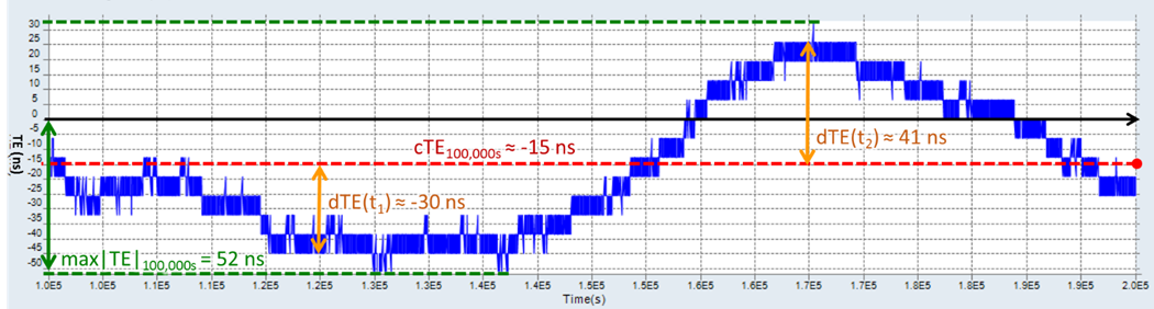
Figure 1. Actual absolute TE graph representing the theoretical concept of cTE and dTE. (Total time: 100,000s)

“Measuring” cTE?

The TE=cTE+dTE “formula” seems to imply that, if we can measure cTE(t) and dTE(t), then we could calculate TE(t). However, in reality, it is the exact opposite. All we can Measure is the instantaneous TE(t). Once enough TE samples have been measured, one can Calculate the mean cTE and then Estimate dTE from it. That is, you would need a very reliable cTE calculation in order to estimate dTE fairly accurately. From one direct measurement (TE) we have created or inferred two indirect parameters, using simple math.

Since cTE is defined as the mean TE value over a “long” observation interval, a 1000s sliding measurement window seems to be considered appropriate within the telecommunications sector. Good enough to average sufficient TE samples to filter the phase noise out and identify that constant cTE component (in just 16 minutes and 40 seconds). A “sliding window” means that the test and measurement system (instrument, meter) continuously averages the last N samples (1000s in this case) to calculate the current cTE (e.g., calculated once every second). Here are some real-life examples of that approach, using measurements from the physical 1PPS output of a GNSS-disciplined clock.

Figure 2. Within this single observation window, one can easily visualize a constant offset, as the average value. cTE ≈ 85.7 ns

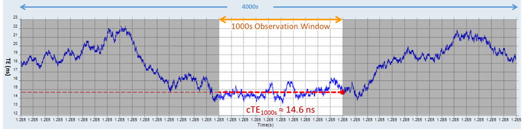
Figure 3. This is another intuitive example of a different 1000s observation window, with its mean value. cTE ≈ 14.6 ns

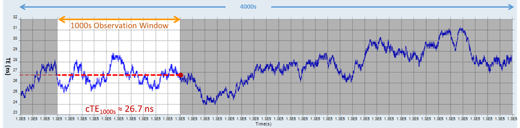
Figure 4. This observation window looks a bit noisier, but one can still visualize its mean value at cTE ≈ 26.7 ns

In certain cases, it is not clear whether there is any constant element within an observation window, nonetheless the algorithm will still output a mean value, based on the last 1000 seconds being processed. For example, when there is a frequency offset component or frequency drift present in the TE behavior (permanent or temporary), like frequency offsets constantly applied by the disciplining loop to correct phase errors and maintain 1PPS alignment.

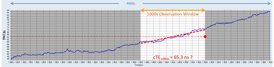
Figure 5. The math calculation still gives a cTE ≈ 65.3 ns result, although there is nothing inherently constant in this window.

However, what if all those traces and values came from a single TE(t) measurement? All made within 24 hours and part of one continuous TE measurement, from the same DUT: A GPS-disciplined Oscillator (GPSDO) device under test. The only difference between them are the individual observation windows selected for each example. The following graph shows 24-hour worth of TE data and identifies all the individual measurement windows described earlier.

Figure 6. 24-hour view of the TE measurements used to extract all the previous cTE examples.

Having cTE values varying from 14 to 86 ns, would imply that the so-called “Constant” TE may not be that constant after all. At least not for short observation intervals, such as 1000s. That is, if the oversimplified concept of TE is used to quickly “measure” cTE in the morning, users may get one set of values. If they “measure” it again in the evening, they could get something completely different. Which value would one use to identify, compensate or fix a problem? Note that the dotted red line representing the overall mean value (e.g., 24h) are just presented as a visual reference. Its output is actually a single average value calculated at the end of the observation window (represented by a red dot).

Some may question whether the GPSDO under test may have been going through its disciplining process, which could justify the phase changes and invalidate the results. However, the answer is NO. The GNSS clock was already in steady locked state, doing its job by trying to keep its time aligned, based on the information it continuously received from satellites. We should also keep in mind that the TE measured is actually relative, a combination of the TE of the DUT and TE of the REF being used, which includes phase errors from both. In the spirit of this discussion:

TE = cTE-cTE+dTE-dTE

So, where did the idea of a 1000s observation window come from? Most likely from controlled lab environments and simulations. Although, it may also have something to do with the convenience of instant gratification (that urge of getting results quickly) and not having to way for a couple of days to complete each test. The problem is that those who provide such guidance often fail to explain their reasoning behind it or any of the trade-offs (e.g., extending the use of 1000s sliding windows for field testing). Sure, one could certainly consider spending one hour measuring TE, most likely getting a somewhat constant cTE value, writing it down on a report, walk away and moving on. But that should not be the point.

When talking about measuring Wander on precision clocks, with accuracies and stability in the order of parts-per-billion (1E-9) or trillion (10E-12), everything happens very slowly. Patience, preparation and dedication are required in order to get valid useful measurements and perhaps good cTE estimates. We need to start by knowing the dynamics of the system under test in order to figure out a reasonable observation window (e.g., PRTC, Grandmaster, PTP link, Boundary clock, Slave clock, GNSS clock, etc.).

We are talking about observation times long enough to capture the most complete or typical system cycle possible (or practical). For example:

• If the DUT is a GPSDO or PRTC, then the total observation time should probably be >1 day to capture the day and night ionospheric contributions, as well as hot and cold temperatures, etc.
• If the DUT is a PTP link, then the total observation time may be >1 day to cover high and low traffic, business-oriented packets during the day vs. streaming-oriented packets in the evening, hot and cold temperatures, etc.

A Real Life (Practical) Example

For example, here is the same measurement data from the GPSDO DUT in question, showing four days’ worth of TE data (still the same test). Longer tests not only provide a better chance of approximating the “true” cTE (one that can be used to “calibrate” or make corrections), it also provides a better idea of the dTE range and MTIE. Most importantly, it provides a better idea of the system’s dynamics.

Figure 7. 4-day 1PPS output TE trace from the GPSDO under test, showing daily time offset variations.

Although that system barely passed the G.8272 PRTC mask, this particular example clearly shows the effects of day/night and high/low-temp cycles. This test was performed in late summer with moderately hot days and cooler nights. At 7:00 pm the building’s HVAC turns itself off during weekdays (first and last days) and stays off during weekends (the two days in the middle).

Perhaps only human eyes (not formulas) can be aware of the context of each test scenario, filter out impairments and visually identify the true mean error floor. The TE data clearly shows the effects of the environment heating up at noon and cooling down at midnight, by a few degrees. That is actually useful and actionable information. Something that can be used to address the issue and improve the system.

Mathematically speaking, the overall TE average of that system, as it is, would be around 40 ns. However, based on a simple visual analysis, we would consider it to be around 18 ns (green line), which is the mean delay that should remain once the temperature problem is addressed, by moving the DUT to a controlled temperature room (equipment room) and adjusting its time constant, as suggested by the manufacturer’s support team. (Refer to Annex A for more details about its final performance.)

Would a four-day monitoring be good recommendation? It all depends. One needs to know the application, environment, the dynamics of the system under test and the reason why we need to know cTE or TE in the first place. Once that is all clear, the measurement requirement may become obvious.

In this particular case, calculating cTE and estimating dTE would not add any value. It is the actual TE(t) trace the one that tells the story and (with experience) technicians could use to infer how to troubleshoot the system and improve their performance, for example:

1. Better temperature control for the DUT.
2. Adjust the disciplining loop time constant.
3. If the GNSS receiver supports multiple satellite systems and or multiple bands, make sure to enable them and verify that the antenna supports them (multi-band operation can help compensate the ionospheric effects and improve the day/night conditions).
4. Now with a cleaner more stable TE trace, then calculate and apply required the time error correction. 

One More Example

For further discussion on cTE usefulness, Figure 8 shows another field test example of the TE from a physical 1PPS clock output and the cTE calculations, using the two different rolling windows and the overall mean value (24h). As expected, the red cTE with 1000s window shows very little difference from the original TE (blue) and even the green cTE with 10000s window struggles to maintain any constant value for an hour. In any case, the variations seem too high to be useful for any practical purposes or to be called “constant” at all!

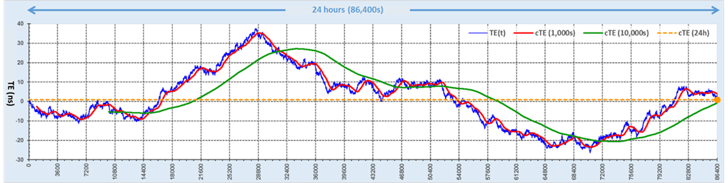
Figure 8. Example of TE(t) and its corresponding rolling cTE(t), calculated with different observation windows.

There should be a good reason why you are being told that you need to know the cTE (as currently defined). Perhaps because you may want to fix it, by inserting an opposite phase offset (calibrate it out), so your system has a better chance of staying within the TE limits during high traffic events, in winter, summer, rainy, snow or sunny days. Based on the actual data and calculations above, the cTE doesn’t seem to be doing a good job at it.

What About dTE?

Figure 8 already confirmed that cTE can actually be a very variable cTE(t) function, which is remarkably close to the original TE(t), with just a few nanoseconds difference. Now, if we take those cTE calculations for granted and use their values to calculate dTE(t)=TE(t)-cTE(t), we arrive to another surprising result.

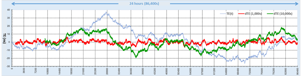
Figure 9. dTE(t)=TE-cTE calculated from the data in Figure 8. Dynamic dTE (red) looks surprisingly constant.

dTE seems to be behaving more like a constant. Although it is not what we were originally told, dTE just seems to be doing a very good job at isolating the high frequency noise (high pass filter).

What if dTE is used (irresponsibly) and the red ±5ns dTE graph alone is presented to you? At first glance it may look like the clock under test is much more stable than it actually is (the actual TE data tells us that it is 6 ±32 ns). So, if TE already tells the full and true story of the DUT, why would we need cTE or dTE?

Conclusion

We need to fully understand what cTE really is and what to expect from it, in order to know when to use it and how it could help us improve our network and timing sources. Always keep in mind that cTE may not be a constant and that it can’t be measured directly. Also keep in mind that this article focuses on physical timing signals and does not address potential applicability of dTE and cTE at the logical level (protocol/packet timestamping and latency).

Are the cTE concept and values useful? Not sure. But it certainly has some limitations that we need to be aware of. It may only be somewhat accurate in determining the required delay compensation for extremely stable systems and under controlled lab environments.

Get to know the system’s dynamics in order to identify the proper observation window and total test time required for a good test. Then weight that against your practical allocation. For example, do you really have 24, 48, 72 or 96 hours to test a PRTC, GPSDO or link? If not, then embrace your reality, adapt your process to it and acknowledge any trade-offs.

Some may still argue that cTE is needed in order to know the constant Delay (or Time Offset) of a system. However, the true system delay may be closer to the minimum delays measured (e.g., caused by cables, fibers, bare electronics delays, buffers, etc.) and they are reflected as negative Time Error (delays). For example, in the packet network that would be the true lucky packets’ latency times, since information can’t travel any faster or arrive earlier.

When measuring or verifying Precision Timing devices or systems, we prefer to stick to the good-old TE and MTIE, because they provide the whole picture, full of actionable information. Something that can be used to fix or improve the settings and hence the synchronization quality of the system. For example, from TIE or TE data we can easily identify and calculate frequency offset, with great accuracy. Then that information can be used to remove it by calibrating (adjusting) the oscillator. That can’t be said for many other acronyms people usually hear at conferences and then start repeating around, for no apparent reasons.                                                                      

Keep in mind that, as we zoom in into the nanosecond scale, used for Precision Timing, nothing is steady or constant anymore. Also, timing references available to regular uses, have time error of their own and those will be embedded in your measurement results. When working outside of controlled labs, you have to embrace those facts and account for the uncertainties.

Perhaps this paper does not provide any specific answers, however we certainly hope it has raised a few questions and pointed you in the right direction, so you can investigate, evaluate and question the usefulness of the cTE, dTE, as well as other concepts, and take them for what they really are, considering any caveats or compromises as you decide whether to apply them into your test and troubleshooting procedures or not.

Annex A. Resulting GPSDO Performance Improvements

Figure 7 showed the fairly good, but not good enough, performance of a single-band GPS-disciplined clock (PRTC) and this section has been added to close the loop on that test case, as it was used as a real-life practical example.

Although it barely passed the PRTC mask at first, a simple visual inspection of the original TE graph showed that something was not quite right and that there was room for improvement. The first hint was the cyclical nature of the TE variations, which the timeline identifies as a daily cycle. That in turn leads to suspects like day/night ionospheric variations and significant room temperature changes. It shows that the direct TE measurement is a very powerful tool on its own.

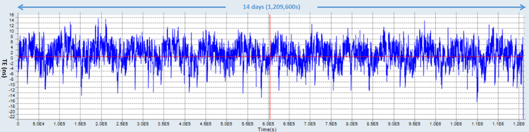
After contacting the manufacturer’s customer support team, they suggested adjusting the time constant (TC) and not using the default settings that came programmed in the brand new Rb GPSDO being used as a PRTC. An 18 ns phase compensation was also applied, based on the assumption (educated guess) explained earlier. The 14-day TE results below show the resulting improvements. It has come down to TE ≈ 1 ±15 ns, from its original 38 ±48 ns.

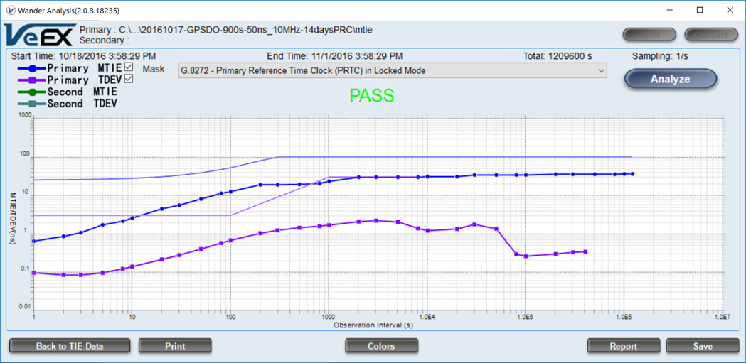
Its G.8272 PRTC mask validation, over a 14-day test, also improved significantly.

Further stability improvements are also expected after the system is moved into the equipment room, which has a more controlled environment.

This goes to show that the TE data provides actionable information, which can be used to troubleshoot, fix and improve the system under test. It is our opinion that TE is a far more practical value for real-life field applications.

Abbreviations & Acronyms

1588v2 - IEEE 1588-2008 standard

1PPS - One Pulse Per Second (its rising edges indicate a beginning of new standard seconds)

cTE - Constant Time Error

dTE - Dynamic Time Error

DUT - Device (or System) Under Test

GNSS - Global Navigation Satellite Systems (often refers to the receivers used to extract standard timing)

GPS - Global Positioning System (the most prevalent GNSS)

GPSDO - GPS Disciplined Oscillator or GPS Clock

HVAC - Heating, Ventilating and Air Conditioning system

ITU-T - International Telecommunication Union - Telecommunication standardization sector

MTIE - Maximum Time Interval Error (maximum peak-to-peak TE or TIE)

NE - Network Element/Equipment

NEM - Network Equipment Manufacturer

PDV - Packet Delay Variation

ppb - Parts per billion (1.0E-9)

ppm - Parts per million (1.0E-6)

ppt - Parts per trillion (1.0E-12)

PRC - Primary Reference Clock (Frequency only)

PRTC - Primary Reference Time Clock (with 1PPS timing and ToD output)

PTP - Precision Timing Protocol (IEEE 1588v2)

REF - Reference Clock (often a traceable PRTC)

T&M - Test and Measurement (industry or equipment)

TDEV - Time Deviation

TE - Time Error

TIE - Time Interval Error

Related Test solutions

• RXT Modular Test Platform
• TX300s Advanced Multi-Service Test Set